This might be one of my most liked papers that probably reveals the essence of graph convolution. It is published on TMLR and is selected as an Oral Presentation at LoG2024 TMLR Track. In this paper, we propose that graph convolution can be viewed as a specialized form of Mixup.

arXiv

1. TL;DR

This paper builds the relationship between graph convolution and Mixup techniques.

• Graph convolution aggregates features from neighboring samples for a specific node (sample).
• Mixup generates new examples by averaging features and one-hot labels from multiple samples.

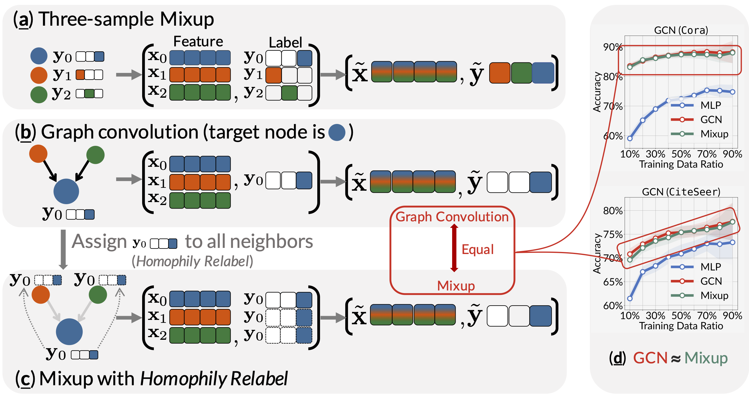
The two share one commonality that information aggregation from multiple samples. We reveal that, under two mild modifications, graph convolution can be viewed as a specialized form of Mixup that is applied during both the training and testing phases if we assign the target node's label to all its neighbors.

2. Graph Convolution ≈ Mixup

Graph Neural Networks have recently been recognized as the de facto state-of-the-art algorithm for graph learning. The core idea behind GNNs is neighbor aggregation, which involves combining the features of a node's neighbors. Specifically, for a target node with feature ${𝒙}_{𝑖}$, one-hot label ${𝒚}_{𝑖}$, and neighbor set ${𝒩}_{𝑖}$, the graph convolution operation in GCN is essentially as follows:

$$\left(\widetilde{𝒙},\widetilde{𝒚}\right)=\left(\frac{1}{\left|{𝒩}_{𝑖}\right|}\sum _{𝑘\in {𝒩}_{𝑖}}{𝒙}_{𝑘},{𝒚}_{𝑖}\right)$$

In parallel, Mixup is proposed to train deep neural networks effectively, which also essentially generates a new sample by averaging the features and labels of multiple samples:

$$\left(\widetilde{𝒙},\widetilde{𝒚}\right)=\left(\sum _{𝑖=1}^{𝑁}{𝜆}_{𝑖}{𝒙}_{𝑖},\sum _{𝑖=1}^{𝑁}{𝜆}_{𝑖}{𝒚}_{𝑖}\right),\text{ s.t. }\sum _{𝑖=1}^{𝑁}{𝜆}_{𝑖}=1$$

where ${𝒙}_{𝑖}$/${𝒚}_{𝑖}$ are the feature/label of sample $𝑖$. Mixup typically takes two data samples ($𝑁=2$).

The above two equations highlight a remarkable similarity between graph convolution and Mixup, i.e., the manipulation of data samples through averaging the features. This similarity prompts us to investigate the relationship between these two techniques as follows:

In this paper, we answer this question by establishing the connection between graph convolutions and Mixup, and further understanding the graph neural networks through the lens of Mixup. We show that graph convolutions are intrinsically equivalent to Mixup by rewriting as follows:

$$\begin{array}{cc}\left(\widetilde{𝒙},\widetilde{𝒚}\right)& =\left(\frac{1}{\left|{𝒩}_{𝑖}\right|}\sum _{𝑘\in {𝒩}_{𝑖}}{𝒙}_{𝑘},{𝒚}_{𝑖}\right)\\ & =\left(\sum _{𝑘\in {𝒩}_{𝑖}}\frac{1}{\left|{𝒩}_{𝑖}\right|}{𝒙}_{𝑘},\sum _{𝑘\in {𝒩}_{𝑖}}\frac{1}{\left|{𝒩}_{𝑖}\right|}{𝒚}_{𝑖}\right)\\ & =\left(\sum _{𝑘\in {𝒩}_{𝑖}}{𝜆}_{𝑖}{𝒙}_{𝑘},\sum _{𝑘\in {𝒩}_{𝑖}}{𝜆}_{𝑖}{𝒚}_{𝑖}\right)\end{array}$$

where ${𝜆}_{𝑖}=\frac{1}{\left|{𝒩}_{𝑖}\right|}$, and ${𝒙}_{𝑖}$ and ${𝒚}_{𝑖}$ are the feature and label of the target node ${𝑛}_{𝑖}$.

This above equation states that graph convolution is equivalent to Mixup if we assign the ${𝒚}_{𝑖}$ to all the neighbors of node ${𝑛}_{𝑖}$ in set ${𝒩}_{𝑖}$.

3. Experiments

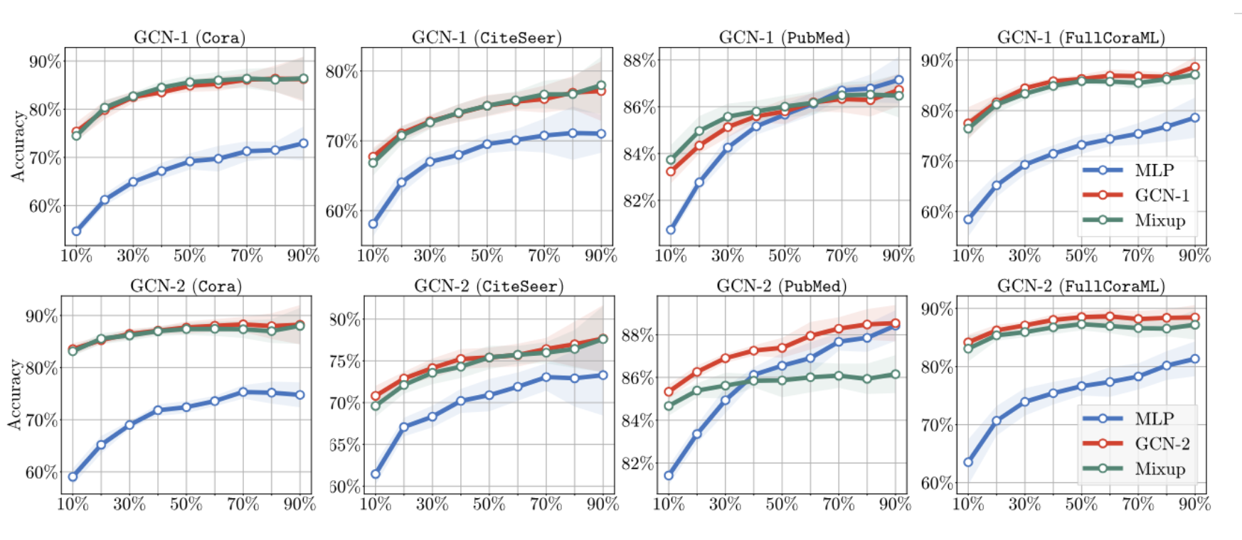
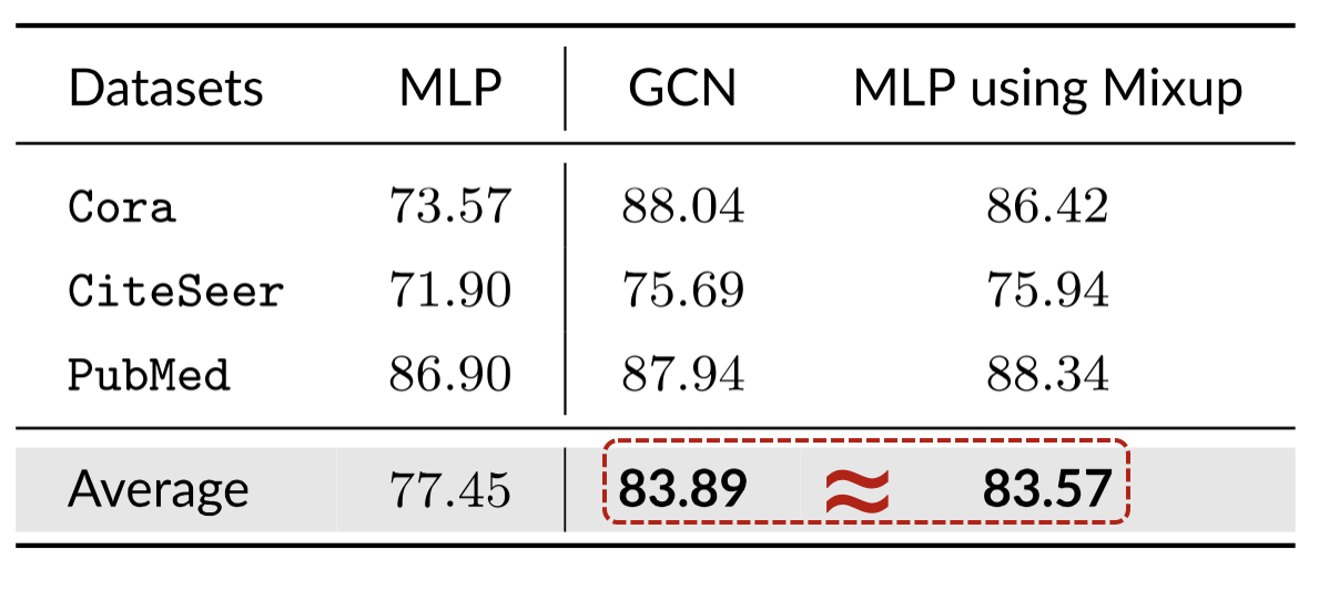
The experiments with the public split on Cora, CiteSeer, and Pubmed datasets and the results are shown in the following table. The results show that MLP with mixup can achieve comparable performance to the original GCN.

We experimented with different data splits of train/validation/test (the training data ratio span from $10\%-90\%$).

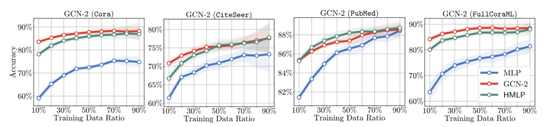
With the test-time mixup (details in the paper), the MLPs with mixup can achieve comparable performance to the original GCN.