Softmax and its triton implementation
  • 10/19/2024
  • Xiaotian Han

  • background

    The softmax function is a fundamental operation in deep learning that converts vectors of real numbers into probability distributions. This blog post explores the softmax function’s implementation and optimization using Triton, a programming framework for efficient GPU computations.

    TL;DR
    • dive into softmax, from math to implementation, from vector to matrix.
    • torch and triton implementations, with reference code and speed comparison.

    The softmax function transforms an input vector into a probability distribution where all elements sum to 1.

    softmax - vector form

    \[\mathbf{o}_i = \mathrm{softmax}(\mathbf{x}_i) = \frac{e^{\mathbf{x}_i}}{\sum_{j=1}^{d} e^{\mathbf{x}_j}}\]

    where:

    • \(\mathbf{x} \in \mathbb{R}^d\): input vector.
    • \(\mathbf{o} \in \mathbb{R}^d\): output vector, probability distribution.

    gradient of softmax (vector form)

    We will compute gradients \(\frac{\partial L}{\partial \mathbf{x}}\) given \(\frac{\partial L}{\partial \mathbf{o}}\), where \(L\) is loss function, \(\mathbf{o}\) is softmax output.

    Jacobian matrix

    softmax is a vector function, the Jacobian matrix is the matrix of all partial derivatives:

    \[\frac{\partial \mathbf{o}}{\partial \mathbf{x}} = \mathbf{J} \;=\; \begin{bmatrix} \frac{\partial \,\mathbf{o}_1}{\partial \,\mathbf{x}_1} & \frac{\partial \,\mathbf{o}_1}{\partial \,\mathbf{x}_2} & \dots & \frac{\partial \,\mathbf{o}_1}{\partial \,\mathbf{x}_d} \\ \frac{\partial \,\mathbf{o}_2}{\partial \,\mathbf{x}_1} & \frac{\partial \,\mathbf{o}_2}{\partial \,\mathbf{x}_2} & \dots & \frac{\partial \,\mathbf{o}_2}{\partial \,\mathbf{x}_d} \\ \vdots & \vdots & \ddots & \vdots \\ \frac{\partial \,\mathbf{o}_d}{\partial \,\mathbf{x}_1} & \frac{\partial \,\mathbf{o}_d}{\partial \,\mathbf{x}_2} & \dots & \frac{\partial \,\mathbf{o}_d}{\partial \,\mathbf{x}_d} \end{bmatrix}.\]

    For softmax, the derivative has two cases:

    1. when \(i = j\), consider \(\mathbf{o}_i = \frac{e^{\mathbf{x}_i}}{\sum_{j=1}^{d} e^{\mathbf{x}_j}}\),

      \[\begin{aligned} \displaystyle \frac{\partial \mathbf{o}_i}{\partial \mathbf{x}_i} &= \frac{ \frac{\partial \left( e^{\mathbf{x}_i} \right)}{\partial \mathbf{x}_i} \cdot \sum_{j=1}^{d} e^{\mathbf{x}_j} - \frac{\partial \left( \sum_{j=1}^{d} e^{\mathbf{x}_j} \right)}{\partial \mathbf{x}_i} \cdot e^{\mathbf{x}_i} }{\left( \sum_{j=1}^{d} e^{\mathbf{x}_j} \right)^2} \\ \displaystyle & = \frac{e^{\mathbf{x}_i} \cdot \sum_{j=1}^{d} e^{\mathbf{x}_j} - e^{\mathbf{x}_i} \cdot e^{\mathbf{x}_i}}{\left( \sum_{j=1}^{d} e^{\mathbf{x}_j} \right)^2} \\ & = \frac{e^{\mathbf{x}_i}}{\sum_{j=1}^{d} e^{\mathbf{x}_j}} \left( 1 - \frac{e^{\mathbf{x}_i}}{\sum_{j=1}^{d} e^{\mathbf{x}_j}} \right) \\ & = \mathbf{o}_i (1 - \mathbf{o}_i) \end{aligned}\]
    2. similarly, when \(i \neq j\):

    \[\frac{\partial \mathbf{o}_i}{\partial \mathbf{x}_j} = -\mathbf{o}_i \mathbf{o}_j\]

    Thus, \((i,j)\)-th element in Jacobian matrix will be:

    \[\mathbf{J}_{ij} = \mathbf{o}_i (\delta_{ij} - \mathbf{o}_j)\]

    where \(\mathbf{J}\) has shape \([d \times d]\) and \(\delta_{ij}\) is the Kronecker delta, which is 1 if \(i = j\) and 0 otherwise.

    In matrix form, the Jacobian of the softmax is:

    \[\mathbf{J} = \mathrm{diag}(\mathbf{o}) - \mathbf{o}\mathbf{o}^\top\]

    where:

    • \(\mathbf{o}\) is the output of softmax, the shape is \([d]\).
    • \(\mathrm{diag}(\mathbf{o})\) is a diagonal matrix of \(\mathbf{o}\), the shape is \([d \times d]\).
    • \(\mathbf{o}\mathbf{o}^\top\) is the outer product of \(\mathbf{o}\) with itself, the shape is \([d \times d]\).

    gradient of \(\frac{\partial L}{\partial \mathbf{x}}\)

    Given \(\frac{\partial L}{\partial \mathbf{o}}\), we can compute \(\frac{\partial L}{\partial \mathbf{x}}\) using the Jacobian matrix:

    \[\frac{\partial L}{\partial \mathbf{x}} = \frac{\partial \mathbf{o}}{\partial \mathbf{x}} \cdot \frac{\partial L}{\partial \mathbf{o}} = \mathbf{J}^{\top} \cdot \frac{\partial L}{\partial \mathbf{o}}\]

    where \(\frac{\partial L}{\partial \mathbf{o}}\) has shape \([d]\), \(\mathbf{J}^{\top}\) has shape \([d \times d]\), and \(\frac{\partial L}{\partial \mathbf{x}}\) has shape \([d]\).

    avoid explicit Jacobian

    Consider the matrix multiplication:

    \[\underbrace{\frac{\partial L}{\partial \mathbf{x}}}_{(d,)} = \underbrace{\mathbf{J}^{\top}}_{(d,d)} \cdot \underbrace{\frac{\partial L}{\partial \mathbf{o}}}_{(d,)}\]

    For the \(i\)-th element of \(\frac{\partial L}{\partial \mathbf{x}}\), we can decompose the computation:

    \[\begin{aligned} \frac{\partial L}{\partial \mathbf{x}_i} &= \sum_{j=1}^{d} \mathbf{J}_{ij} \frac{\partial L}{\partial \mathbf{o}_j} \\ &= \underbrace{\mathbf{o}_i(1-\mathbf{o}_i) \frac{\partial L}{\partial \mathbf{o}_i}}_{j=i} + \underbrace{-\mathbf{o}_i \sum_{j\ne i}\mathbf{o}_j \frac{\partial L}{\partial \mathbf{o}_j}}_{j\ne i} \\ & = \mathbf{o}_{i}\left(\frac{\partial L}{\partial \mathbf{o}_{i}}-\sum_{j=1}^{d}\mathbf{o}_{j}\frac{\partial L}{\partial \mathbf{o}_{j}}\right) \end{aligned}\]

    This leads to an efficient vector form:

    \[s_{grad}=\left( \mathbf{o} \odot \frac{\partial L}{\partial \mathbf{o}}\right)_{sum}\] \[\frac{\partial L}{\partial \mathbf{x}}= \mathbf{o} \odot\left(\frac{\partial L}{\partial \mathbf{o}}-s_{grad}\right)\]

    softmax - batch form

    \(\mathbf{X}\): A batch of input vectors.

    \[\mathbf{X} \in \mathbb{R}^{N \times d}\]

    where:

    • \(N\) is batch size.
    • \(d\) is vector dimension.

    forward pass

    \[\mathbf{E} = e^\mathbf{X}\] \[\mathbf{s} = \sum_{j=1}^{d} e^{\mathbf{X}_{ij}}\] \[\mathbf{O} = \frac{ \mathbf{E} }{ \mathbf{s} }\]

    where \(\mathbf{E} \in \mathbb{R}^{N \times d}\), \(\mathbf{s} \in \mathbb{R}^{N \times 1}\), \(\mathbf{O} \in \mathbb{R}^{N \times d}\).

    backward pass

    We have gradient with respect to softmax output:

    \[\frac{\partial L}{\partial \mathbf{O}} \in \mathbb{R}^{N \times d}\]

    we compute the gradient:

    \[\mathbf{s}_{grad} = \left( \mathbf{O} \odot \frac{\partial L}{\partial \mathbf{O}} \right)_{row\_sum} \in \mathbb{R}^{N \times 1}\]

    where \(\mathbf{O}\) has size \([N \times d]\), and \(\frac{\partial L}{\partial \mathbf{O}}\) has size \([N \times d]\).

    \[\frac{\partial L}{\partial \mathbf{X}} = \mathbf{O} \odot \left( \frac{\partial L}{\partial \mathbf{O}} - \mathbf{s}_{grad} \right)\]

    where \(\frac{\partial L}{\partial \mathbf{X}} \in \mathbb{R}^{N \times d}\) and \(\mathbf{O} \in \mathbb{R}^{N \times d}\) and \(\mathbf{s}_{grad} \in \mathbb{R}^{N \times 1}\) will be broadcasted to \(\mathbb{R}^{N \times d}\).

    implementation

    In practice, we subtract the maximum value from each row before applying exp() to prevent numerical overflow:

    real forward pass

    For input \(\mathbf{X} \in \mathbb{R}^{N \times d}\):

    \[\begin{aligned} \mathbf{X}_{max} &= \max(\mathbf{X}) \in \mathbb{R}^{N \times 1}\\ \mathbf{E} &= e^{\mathbf{X} - \mathbf{X}_{max}} \\ \mathbf{s} &= \sum_{j=1}^{d} e^{\mathbf{X}_{ij} - \mathbf{X}_{max}} \\ \mathbf{O} &= \frac{ \mathbf{E} }{ \mathbf{s} } \end{aligned}\]

    real backward pass

    we have \(\frac{\partial L}{\partial \mathbf{O}} \in \mathbb{R}^{N \times d}\) and cached \(\mathbf{O} \in \mathbb{R}^{N \times d}\)

    \[\begin{aligned} \mathbf{s}_{grad} &= \left( \mathbf{O} \odot \frac{\partial L}{\partial \mathbf{O}} \right)_{row\_sum} \\ \frac{\partial L}{\partial \mathbf{X}} &= \mathbf{O} \odot \left( \frac{\partial L}{\partial \mathbf{O}} - \mathbf{s}_{grad} \right) \end{aligned}\]

    a real example

    give a real example to show how to implement softmax and its backward pass in pytorch and triton.

    forwards pass is as follows:

    \[X = \begin{bmatrix} 1.0 & 2.0 & 3.0 \\ 1.0 & 3.0 & 5.0 \end{bmatrix}\] \[X_{max} = \begin{bmatrix} 3.0 \\ 5.0 \end{bmatrix}\] \[X - X_{max} = \begin{bmatrix} -2.0 & -1.0 & 0.0 \\ -4.0 & -2.0 & 0.0 \end{bmatrix}\] \[E = e^{X - X_{max}} = \begin{bmatrix} e^{-2.0} & e^{-1.0} & e^{0.0} \\ e^{-4.0} & e^{-2.0} & e^{0.0} \end{bmatrix}\] \[E = \begin{bmatrix} 0.1353 & 0.3679 & 1.0000 \\ 0.0183 & 0.1353 & 1.0000 \end{bmatrix}\] \[S = \begin{bmatrix} 1.5032 \\ 1.1536 \end{bmatrix}\] \[O = \frac{E}{S} = \begin{bmatrix} 0.0900 & 0.2447 & 0.6652 \\ 0.0159 & 0.1173 & 0.8668 \end{bmatrix}\]

    backward pass is as follows: \(dO = \begin{bmatrix} 0.1 & 0.2 & 0.7 \\ 0.2 & 0.3 & 0.5 \end{bmatrix}\)

    \[\begin{aligned} s_{grad} &= \begin{bmatrix} 0.0900 \times 0.1 & 0.2447 \times 0.2 & 0.6652 \times 0.7 \\ 0.0159 \times 0.2 & 0.1173 \times 0.3 & 0.8668 \times 0.5 \end{bmatrix}\\ &= \begin{bmatrix} 0.0090 & 0.0489 & 0.4656 \\ 0.0032 & 0.0352 & 0.4334 \end{bmatrix} \\ &= \begin{bmatrix} 0.2036 \\ 0.2597 \end{bmatrix} \end{aligned}\] \[dX = O \circ \left( dO - s_{grad} \right)\] \[\begin{bmatrix} -0.1036 & -0.0036 & 0.4964 \\ -0.0597 & 0.0403 & 0.2403 \end{bmatrix}\] \[dX = \begin{bmatrix} 0.0900 \times (-0.1036) & 0.2447 \times (-0.0036) & 0.6652 \times 0.4964 \\ 0.0159 \times (-0.0597) & 0.1173 \times 0.0403 & 0.8668 \times 0.2403 \end{bmatrix}\] \[dX = \begin{bmatrix} -0.0381 & -0.0792 & 0.1173 \\ -0.0043 & -0.0202 & 0.0245 \end{bmatrix}\]

    native pytorch implementation

    import torch
    import torch.nn.functional as F
    
    # Custom Forward Pass (Numerically Stable Softmax)
    def softmax_forward(X):
        X_max = torch.max(X, dim=1, keepdim=True)[0]  # Shape: (N, 1)
        E = torch.exp(X - X_max)                     # Shape: (N, d)
        S = torch.sum(E, dim=1, keepdim=True)        # Shape: (N, 1)
        O = E / S                                    # Shape: (N, d)
        return O
    
    # Custom Backward Pass (Gradient Calculation)
    def softmax_backward(dL_dO, O):
        s_grad = torch.sum(O * dL_dO, dim=1, keepdim=True)  # Shape: (N, 1)
        dL_dX = O * (dL_dO - s_grad)                        # Shape: (N, d)
        return dL_dX
    
    # Example Inputs
    X = torch.tensor([[1.0, 2.0, 3.0], [1.0, 3.0, 5.0]], requires_grad=True)
    dL_dO = torch.tensor([[0.1, 0.2, 0.7], [0.2, 0.3, 0.5]])
    
    # Custom Implementation - Forward
    O_custom = softmax_forward(X)
    
    # PyTorch Implementation - Forward
    O_pytorch = F.softmax(X, dim=1)
    
    # Verify Forward Output
    print("Custom Softmax Output:\n", O_custom)
    print("PyTorch Softmax Output:\n", O_pytorch)
    print("Forward Pass Match:", torch.allclose(O_custom, O_pytorch))
    
    # Custom Implementation - Backward
    dL_dX_custom = softmax_backward(dL_dO, O_custom)
    
    # PyTorch Automatic Gradient Calculation
    O_pytorch.backward(dL_dO)  # Computes gradient using PyTorch autograd
    dL_dX_pytorch = X.grad
    
    # Verify Backward Output
    print("\nCustom Gradient w.r.t Input:\n", dL_dX_custom)
    print("PyTorch Gradient w.r.t Input:\n", dL_dX_pytorch)
    print("Backward Pass Match:", torch.allclose(dL_dX_custom, dL_dX_pytorch))
    

    output:

    Custom Softmax Output:
     tensor([[0.0900, 0.2447, 0.6652],
            [0.0159, 0.1173, 0.8668]], grad_fn=<DivBackward0>)
    PyTorch Softmax Output:
     tensor([[0.0900, 0.2447, 0.6652],
            [0.0159, 0.1173, 0.8668]], grad_fn=<SoftmaxBackward0>)
    Forward Pass Match: True
    
    Custom Gradient w.r.t Input:
     tensor([[-0.0381, -0.0792,  0.1173],
            [-0.0043, -0.0202,  0.0245]], grad_fn=<MulBackward0>)
    PyTorch Gradient w.r.t Input:
     tensor([[-0.0381, -0.0792,  0.1173],
            [-0.0043, -0.0202,  0.0245]])
    Backward Pass Match: True
    

    triton implementation

    
    from typing import Optional
    
    import torch
    import triton
    import triton.language as tl
    
    
    @triton.jit
    def softmax_fwd_kernel(
        X,
        O,
        D: tl.constexpr,
        B: tl.constexpr
    ):
        i_n = tl.program_id(0)
        o_d = tl.arange(0, B)
        m_d = o_d < D
    
        X_max = tl.max(tl.load(X + i_n * D + o_d, mask=m_d, other=-float('inf')), 0)
        E = tl.exp(tl.load(X + i_n * D + o_d, mask=m_d, other=-float('inf')) - X_max)
        S = tl.sum(E, 0)
        P = E / S
    
        tl.store(O + i_n * D + o_d, P.to(O.dtype.element_ty), mask=m_d)
    
    
    @triton.jit
    def softmax_bwd_kernel(
        O,
        dO,
        dX,
        D: tl.constexpr,
        B: tl.constexpr
    ):
        i_n = tl.program_id(0)
        o_d = tl.arange(0, B)
        m_d = o_d < D
    
        P = tl.load(O + i_n * D + o_d, mask=m_d, other=0.)
        dP = tl.load(dO + i_n * D + o_d, mask=m_d, other=0.)
        s_grad = tl.sum(P * dP, 0)
        dX_row = P * (dP - s_grad)
    
        tl.store(dX + i_n * D + o_d, dX_row.to(dX.dtype.element_ty), mask=m_d)
    
    
    def softmax_fwd(
        X: torch.Tensor,
        dtype: Optional[torch.dtype] = torch.float
    ) -> torch.Tensor:
        shape = X.shape
        X = X.view(-1, X.shape[-1])
    
        N, D = X.shape
        B = triton.next_power_of_2(D)
    
        O = torch.empty_like(X, dtype=dtype)
        softmax_fwd_kernel[(N,)](
            X=X,
            O=O,
            D=D,
            B=B
        )
        return O.view(*shape)
    
    
    def softmax_bwd(
        O: torch.Tensor,
        dO: torch.Tensor,
        dtype: Optional[torch.dtype] = torch.float
    ) -> torch.Tensor:
        shape = O.shape
        O = O.view(-1, O.shape[-1])
        dX = torch.empty_like(O, dtype=dtype)
    
        N, D = O.shape
        B = triton.next_power_of_2(D)
        softmax_bwd_kernel[(N,)](
            O=O,
            dO=dO,
            dX=dX,
            D=D,
            B=B
        )
        return dX.view(*shape)


    # Test code to verify correctness
    import torch.nn.functional as F
    
    # Example inputs
    X = torch.tensor([[1.0, 2.0, 3.0], [1.0, 3.0, 5.0]], requires_grad=True, device='cuda')
    dP = torch.tensor([[0.1, 0.2, 0.7], [0.2, 0.3, 0.5]], device='cuda')
    
    # Forward pass
    P_triton = softmax_fwd(X)
    P_torch = F.softmax(X, dim=1)
    
    # Verify forward pass
    print( "P_triton:\n", P_triton)
    print( "P_torch:\n", P_torch)
    print("Forward Pass Match:", torch.allclose(P_triton, P_torch))
    
    # Backward pass
    
    dX_triton = softmax_bwd(P_triton, dP)
    P_torch.backward(dP)
    dX_torch = X.grad
    
    # Verify backward pass
    print( "dX_triton:\n", dX_triton)
    print( "dX_torch:\n", dX_torch)
    print("Backward Pass Match:", torch.allclose(dX_triton, dX_torch))


    output:

    P_triton:
     tensor([[0.0900, 0.2447, 0.6652],
            [0.0159, 0.1173, 0.8668]], device='cuda:0')
    P_torch:
     tensor([[0.0900, 0.2447, 0.6652],
            [0.0159, 0.1173, 0.8668]], device='cuda:0', grad_fn=<SoftmaxBackward0>)
    Forward Pass Match: True
    dX_triton:
     tensor([[-0.0381, -0.0792,  0.1173],
            [-0.0043, -0.0202,  0.0245]], device='cuda:0')
    dX_torch:
     tensor([[-0.0381, -0.0792,  0.1173],
            [-0.0043, -0.0202,  0.0245]], device='cuda:0')
    Backward Pass Match: True
    

    speed comparison

    The performance comparison between PyTorch and Triton implementations reveals:
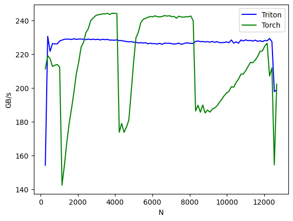
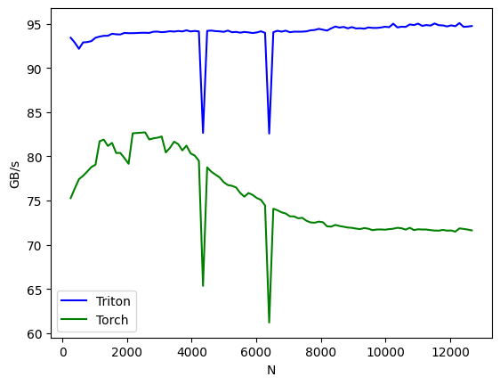
    forward pass
    forward pass
    backward pass
    backward pass

    Results show

    • forward pass: triton implementation is stable, while the PyTorch implementation is faster for most batch sizes but shows fluctuations for a few.
    • backward pass: triton implementation outperforms the pytorch implementation across most batch sizes. (the comparison may not be entirely fair, as triton caches the output \(O\), whereas pytorch’s handling intermediate values is unclear.)

    notions

    symbol shape definition
    \(\mathbf{x}\) \(d\) Input vector
    \(\mathbf{o}\) \(d\) Output vector (probability distribution)
    \(L\) Scalar Loss function
    \(\mathbf{J}\) \(d \times d\) Jacobian matrix
    \(\mathbf{X}\) \(N \times d\) Batch of input vectors (matrix)
    \(\mathbf{O}\) \(N \times d\) Batch output probabilities
    \(\frac{\partial L}{\partial \mathbf{O}}\) \(N \times d\) Gradient w.r.t. output probabilities
    \(\frac{\partial L}{\partial \mathbf{X}}\) \(N \times d\) Gradient w.r.t. input vectors
    \(s_{grad}\) \(N \times 1\) Summation of gradients, \(s_{grad} = (\mathbf{O} \odot \frac{\partial L}{\partial \mathbf{O}})_{sum}\)

    Note:

    • Symbols like \(x\), \(\mathbf{x}\), \(\mathbf{X}\) represent scalars, vectors, or matrices, where uppercase denotes batch forms.
    • \(\mathbf{X}_{:,i}\) denotes a column vector, \(\mathbf{X}_{i,:}\) denotes a row vector, \(\mathbf{X}_{i,j}\) and denote the \((i,j)\)-th element
    • \(\mathbf{x}_i\) denote the \(i\)-th element.